Part 1 established that GBT inference latency is driven by memory access, not arithmetic. The fastest path to lower and more predictable latency, after controlling tree structure, is to reduce the model’s memory footprint. Less data to load means more of it fits in fast local storage, which means fewer stalls, less variance, tighter latency.
The tool for reducing footprint is quantisation: representing numerical values with fewer bits. As an example, Table 1 shows the models used in the STAC-ML ElPopo (electronic trading) benchmark. Moving from a 64-bit float to a 32-bit float halves the memory required for each value, saving 33% of space; a fixed-point representation at 16 bits saves a further 25% on top of that.
.png)
But before reaching for these reductions, it is worth asking: what are the numbers in a GBT model actually doing? Because not all numbers fail the same way when you make them less precise; in a GBT, one type of failure is manageable, and the other is not.
A GBT Model Has Two Distinct Roles for Numbers
Open any trained GBT model and you find two kinds of stored values:
Decision thresholds live at every internal node. They are used in comparisons: is feature 𝑥𝑖 less than threshold 𝑡𝑗? The answer is binary, yes or no, and it determines which branch the input follows next.
Leaf values live at every terminal node. They are the prediction contributions: when an input reaches a leaf, it collects that leaf’s value. The final output is the sum of all collected leaf values across all trees.
These two types of numbers do completely different jobs. Thresholds make routing decisions. Leaf values make numerical contributions. That difference is everything when it comes to quantisation.
What Happens When You Round a Threshold
Rounding a threshold changes a boundary. Instead of asking is 𝑥𝑖 < 1.000001, the model asks is 𝑥𝑖 < 1.0. For most inputs, the answer is the same. But for an input whose feature value sits near the boundary, say 𝑥𝑖 = 1.0000005, the rounding may reverse the comparison, sending the input down the wrong branch.
Here is the critical point: the wrong branch leads to a completely different leaf. The prediction error is not proportional to how much the threshold was rounded. It is proportional to the difference in value between the correct leaf and the leaf the input incorrectly reaches, which can be arbitrarily large.
This is structurally different from quantising a neural network weight. In a neural network, rounding a weight slightly perturbs the output continuously and proportionally. In a GBT, rounding a threshold can teleport an input to an unrelated leaf. The error is discrete and unbounded.
Comparing LightGBM’s native float64 inference against ONNX Runtime’s float32 inference, as Table 2 shows, the RMSE looks fine. The maximum error does not. A 235% prediction error on GBT_A means some outputs are not slightly wrong or directionally wrong; they are wrong by more than double. These cases are rare (0.2% of tests), but in a trading context, a rare catastrophic signal is precisely the failure mode you cannot afford.
.png)
The Fix: Quantise During Training, Not After
The intuitive response is to use higher-precision thresholds. But that sacrifices the memory footprint reduction we were after in the first place.
The correct fix is to quantise the feature data before it enters the training pipeline, and hold that quantisation fixed at inference.
The reasoning is straightforward. Post-training quantisation rounds a float64 threshold to the nearest representable value at the target precision. The boundary moves slightly. Any input whose feature value sits in the gap between the original boundary and the rounded boundary will now take the wrong branch. These “ambiguous inputs” exist whenever the original threshold had sub-tick precision, which is true of virtually every threshold in a model trained on continuous data.
Training-time quantisation eliminates this entirely. If every feature value in the training data is already rounded to the target step size 𝛿, then every candidate split threshold the training algorithm considers lies between two consecutive multiples of 𝛿. No input, whether training or inference, can ever land in the gap that post-training rounding would move a boundary across, because the input grid has no points there. The comparison outcome is identical before and after any further rounding of the threshold.
The resulting model does not approximate float inference at lower precision; it is the correct model at that precision, with zero mismatch.
What Happens When You Round a Leaf Value
Leaf values behave differently because they are additive, not decisive. Rounding a leaf value slightly perturbs the partial sum it contributes. The error accumulates across all trees, but it does so continuously and predictably. No input is rerouted. No catastrophic jump occurs.
This means leaf quantisation is a solvable numerical problem. The required bit-width can be derived analytically from the trained ensemble, using two constraints:
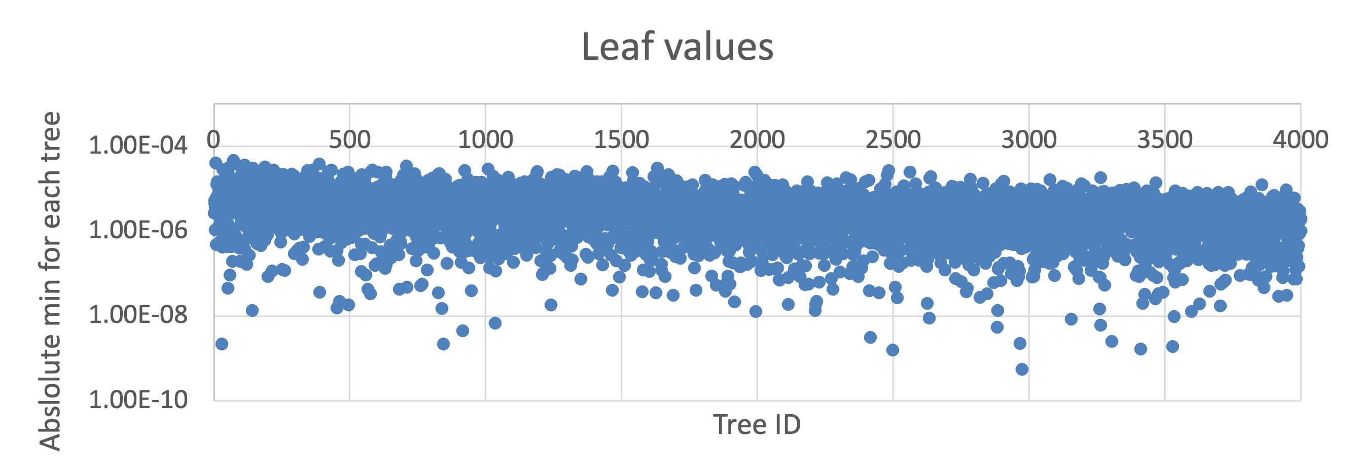
The rounding constraint comes from the smallest leaf values in the ensemble. A leaf value very close to zero requires many fractional bits to represent without being rounded to zero entirely. The required fractional bit-width is:

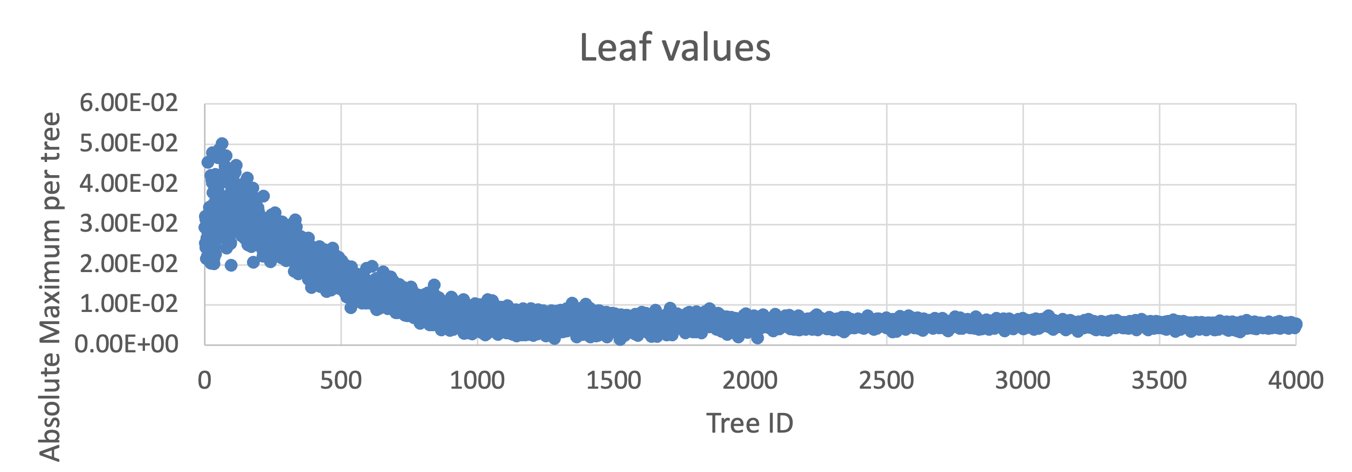
The overflow constraint comes from the largest possible accumulation. In the worst case, every tree contributes its maximum-magnitude leaf. The sum of those maxima must not overflow the accumulator. The required integer bit-width is:

The total required bit-width is 𝑏int +𝑏frac, and it is specific to each model; you compute it from the trained ensemble.
For the STAC-ML GBT models, the analysis gives:
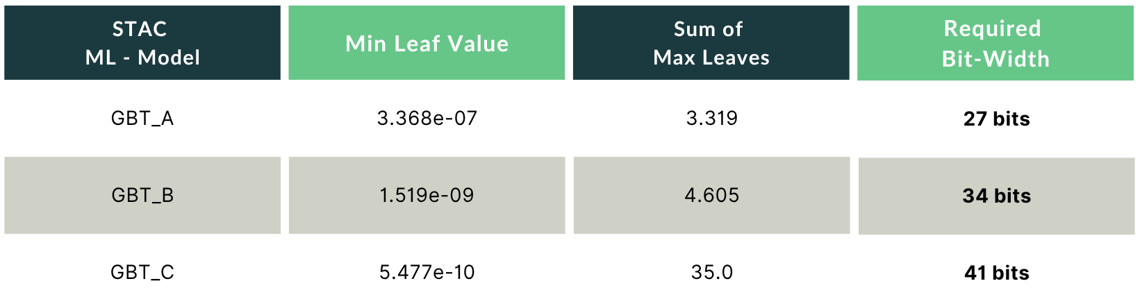
As Table 3 shows, GBT_A is comfortable at 32 bits. GBT_B needs 34, requiring a 64-bit accumulator with careful rounding. GBT_C needs 41 bits, again requiring a 64bit accumulator. The implication is that thresholds and leaf values must be handled at different precisions within the same implementation. The 32-bit figure for thresholds is achievable; for leaves, the required width is model-specific and must be computed, not assumed.
The Full Picture
Putting both analyses together: a correctly quantised GBT model trains on data that has already been quantised to the target threshold precision, and stores leaf values at the bit-width derived analytically from the ensemble’s value distribution. This gives you the full memory footprint reduction without the tail-error catastrophes that naive post-training compression produces.
What quantisation does not give you is deterministic latency. It reduces footprint, which reduces local memory pressure, which narrows the latency distribution. But as long as the computation runs on a general-purpose compute platform, there are sources of variance that no model-level optimisation can eliminate. That is the territory of Part 3.