This series of blog articles works through the problem of achieving low and deterministic inference latency for Gradient Boosted Tree (GBT) models in latency-sensitive trading. The argument is developed across three layers, model structure, numerical representation, and compute architecture, each building on the one before.
Audience. Quantitative developers, infrastructure engineers, and technology decision-makers evaluating ML inference for time-critical trading strategies.
Benchmark data. Numerical examples throughout this series use the STAC-ML benchmark suite, an industry standard set of workloads and reference models for evaluating machine learning inference performance in electronic trading environments.
In this article, we focus on GBT Inference Latency: Why the model itself is a latency variable, and how tree structure and ensemble mapping determine the range of possible execution times.
What a GBT Prediction Actually Does
Before any optimisation, it is worth asking a basic question: what is a GBT prediction, mechanically?
An input arrives as a vector of feature values. The model evaluates each tree in the ensemble: starting at the root, it tests a feature against a threshold, follows the appropriate branch, tests another feature, follows another branch, and continues until it reaches a terminal node, a leaf, and reads off a number. It does this for every tree. The prediction is the sum of all those numbers.
That is the entire computation. A GBT prediction is a routing operation followed by an accumulation. There is no matrix multiplication, no activation function, no attention mechanism. Just a sequence of comparisons and a sum.
This simplicity has an important implication: GBT inference speed is not limited by arithmetic. It is limited by how quickly the model can read the data it needs to perform each comparison.
The Cost of a Single Comparison
Each node in a tree stores two things: a threshold value and two pointers (or index offsets) to child nodes. To traverse the tree, the inference engine must load these values from memory for each node it visits.
The time to load a value from memory is not constant. It depends entirely on where that value lives in the memory hierarchy at the moment of the request. If it is in the compute unit’s fastest local store, access is near-instantaneous. If it is not, the compute unit stalls and waits, potentially for many times longer.
Which tier a value lands in depends on what was accessed recently. Memory systems keep recently-used data close. If a tree was traversed moments ago on similar input, its nodes may still be resident in fast local storage. If the model is large, or if the input exercises an unusual branch not recently visited, the relevant nodes may have been evicted and must be re-fetched from slower memory.

Here is the key point: which path an input takes through a tree depends on the input itself. Different inputs follow different paths, load different nodes, and encounter different memory latency profiles. This is why GBT inference latency is input-data dependent, and why measuring average latency tells you almost nothing about what will happen on a specific input in production.
How Tree Shape Determines Latency Range
The range of possible latency values for a given tree is set by the range of possible path lengths through it, from shortest branch to longest branch.
A perfectly balanced tree of depth 𝑑 has the same path length for every input: exactly 𝑑 comparisons. Every input loads the same number of nodes. Latency is bounded and predictable.
An unbalanced tree has path lengths that vary from shallow to deep depending on which branches were split during training. A single input might traverse 3 comparisons; another might traverse 12. The node accesses are different, the memory access pattern is different, and the latency is different.
XGBoost grows trees level by level, visiting all nodes at depth 𝑘 before any at depth 𝑘 + 1. The result is balanced, symmetric trees with uniform path lengths.
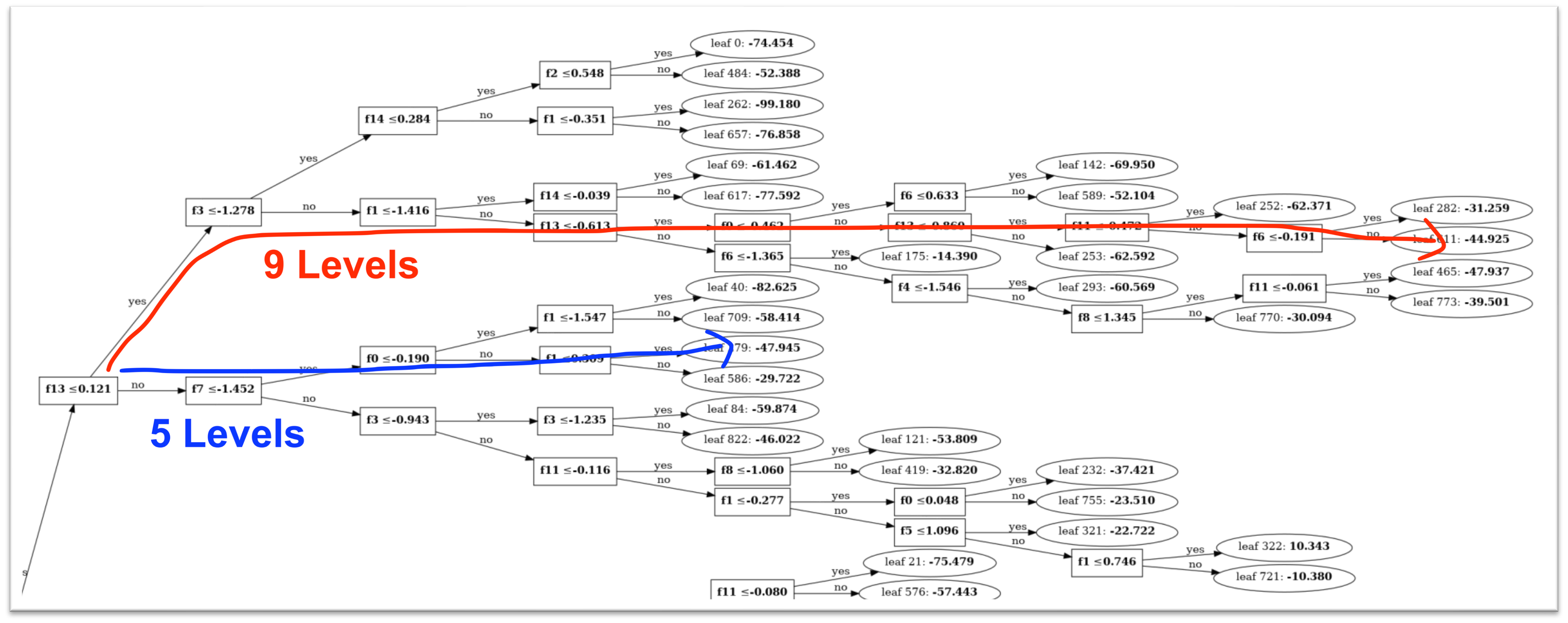
LightGBM grows trees leaf by leaf, always splitting the leaf with the highest loss reduction, regardless of depth. The result is asymmetric trees that often achieve better accuracy with fewer trees, but at the cost of highly variable path lengths. A single LightGBM tree can have leaves at depth 2 sitting next to leaves at depth 15.
For production deployment, this asymmetry is a latency liability. The max_depth parameter in LightGBM directly caps the deepest possible path, converting an open-ended latency range into a bounded one. This is not a regularisation decision; it is a latency contract. Treat it as such.
Choosing max_depth involves a trade-off: shallower trees are less expressive, so you may need more trees to achieve the same accuracy. Profile inference latency at the 99.9th percentile, not the mean, across a range of max_depth values from 4 to 10. You will find a knee in the curve where tail latency stabilises sharply at modest accuracy cost. That knee is your operating point.
From One Tree to an Ensemble
A single tree is fast regardless of depth. The challenge is the ensemble: hundreds or thousands of trees whose outputs must all be computed and summed before a prediction can be returned. The natural approach is parallelism: distribute 𝑁 trees across 𝑃 processing units, each with its own ALU and local memory, and sum the results at the end. A simple model of the cost is:

This model looks clean, but two hidden costs break its simplicity.
The first cost is the reduction term 𝐿reduction. Summing partial results from 𝑃 units requires communication between them. This cost grows with 𝑃 and does not disappear with faster compute; it is a synchronisation cost, and synchronisation is expensive at nanosecond scales.
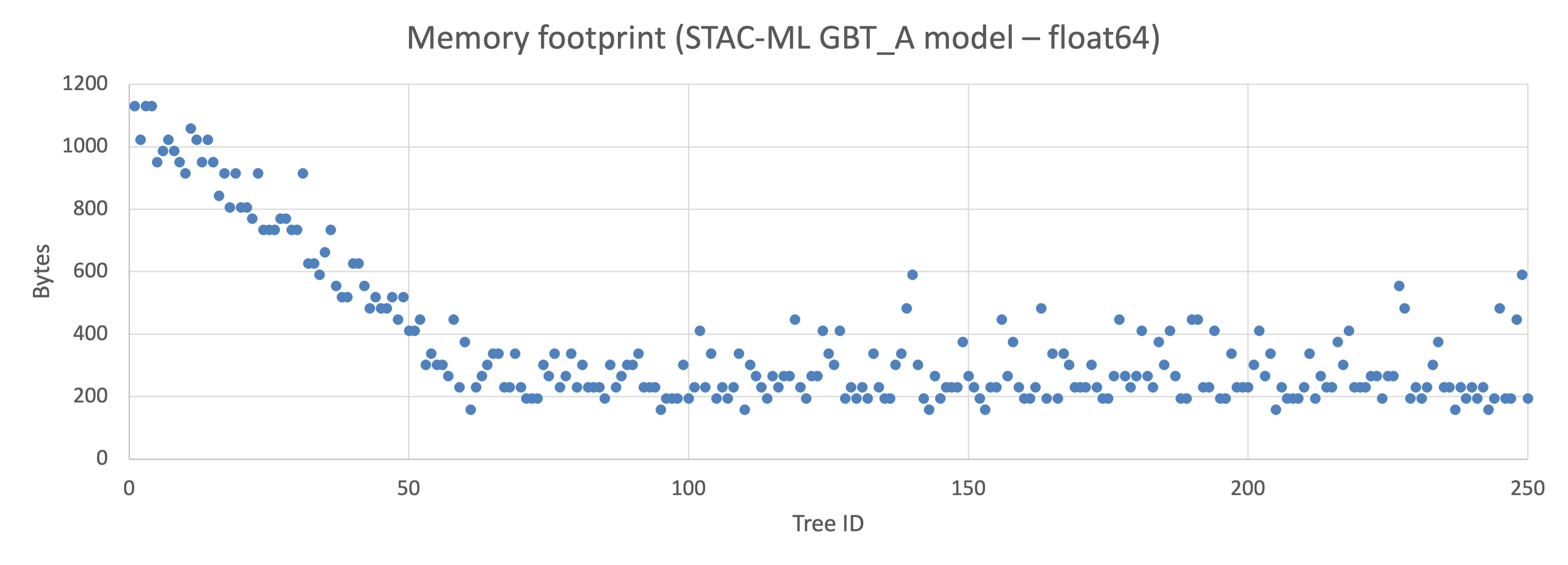
The second cost is that trees are not equal in size. In an uncontrolled LightGBM ensemble, tree memory footprints can vary by orders of magnitude. If trees are assigned round-robin to processing units, some units end up holding small trees that fit entirely in local memory, while others hold large trees that spill into slower memory tiers. Those units are slower. The ensemble latency is then determined by the slowest unit.
The fix is to assign trees to processing units based on their memory footprint, balancing total load rather than tree count.
Setting max_depth helps here too: bounded tree depth means bounded footprint variance, which means the load-balancing problem is more tractable.
What This Gives You
Applying these two structural controls, max_depth and footprint-balanced assignment, changes the latency profile from “highly variable, input-dependent” to “bounded and predictable.” You have not changed what the model computes. You have changed the envelope of how long it takes to compute it.
The remaining source of latency variance is the size of the model itself: how much memory it occupies, and how much of that fits in fast local storage. Reducing that footprint is the subject of Part 2.
Practical Checklist
• Set max_depth on LightGBM models before deployment. A value of 6–8 is a reasonable starting point; tune against 99.9th percentile latency.
• Measure per-tree memory footprints. Assign trees to processing units by total footprint, not tree count.