Parts 1 and 2 worked through what you can control at the model level: tree structure to bound path lengths, quantisation to shrink memory footprint. Done well, these reduce and tighten latency significantly. But they operate within a constraint they cannot remove.
That constraint is the compute platform itself.
To understand why, start with a simple question: in any computation, where does the time go?
Time is spent in three activities. Moving data from where it lives to where it is needed. Executing logic on that data. Synchronising results when multiple units have worked in parallel. Every architecture makes implicit choices about which of these activities dominates; for latency-sensitive inference, those choices matter enormously.
CPU Inference: Fast, but with a Ceiling
With core isolation, NUMA-aware allocation, branch-predictor warming, and vectorised tree traversal, optimised CPU inference is genuinely fast. For a small model on a single isolated core, sub-microsecond latency at the 99th percentile is achievable, competitive with, and in some cases faster than, a PCIe-attached accelerator, because there is no data-transfer overhead. This advantage, however, is specific to the single-model, low-contention scenario described here; it does not generalise to production workloads, as discussed below.
The CPU path requires no additional hardware, integrates via a standard C/C++ or Python API, and is the most cost-effective deployment for models that fit in L2/L3 cache.
The limitation is structural, not a matter of tuning. Interrupts, scheduler preemption, cache eviction by neighbouring processes, and power-management clock adjustments all introduce latency spikes that no user-space optimisation can eliminate. Even on a tuned, isolated core, the observed maximum can exceed the 99th percentile by an order of magnitude. Under concurrent multi-model load, the condition that matters in production, the gap widens further: the last-level cache, memory controller, and interrupt controller are shared across all cores, and contention for these resources pushes worst-case latency to hundreds of microseconds or even milliseconds. At that point, a PCIe-attached accelerator with dedicated memory and a deterministic execution pipeline will typically deliver more predictable latency despite the transfer cost.
Two Ways to Attach an Accelerator
Once the CPU's tail-latency ceiling becomes a binding constraint, the question is how to move inference onto dedicated hardware. There are two fundamentally different ways to do it. They differ not in compute speed but in data movement, and data movement, at nanosecond scales, dominates everything else.
The Offload Architecture (PCIe-Attached Accelerator)
In an offload architecture, the accelerator is a peripheral device connected to the host server via a PCIe bus. The host receives a market data event, assembles the feature vector, transfers it to the accelerator, waits for inference to complete, and receives the result back over PCIe.
The inference latency of this workflow is the sum of three terms: PCIe transfer to accelerator, compute on accelerator, PCIe transfer back. The accelerator compute term can be made very fast. The PCIe terms set the floor.
Benchmark data on a well-tuned server platform with an ultra-low-latency PCIe data handling system illustrates each component of this floor.
The data transfer cost. A full round-trip loopback (host to accelerator and back) adds to this base cost depending on payload size. For the feature vector sizes typical in HFT models (64–1024 features at 4 bytes each), PCIe floor is not a bandwidth limitation but a transaction latency floor set by DMA setup and bus arbitration, a fixed cost per round-trip regardless of how small the payload is.
The concurrency cost. Under many simultaneous parallel transfers, the 99th percentile should remain tightly clustered across all streams. A well-designed PCIe data handling system must arbitrate multi-process access without introducing latency imbalance between competing processes, a critical property for trading systems where multiple strategy threads share the same accelerator card.
The practical consequence for inference is that, for a small model where CPU compute itself takes well under a microsecond, the PCIe round-trip accounts for most of the total offload latency. You have paid for a fast engine and attached it with a connector that costs more than the computation itself. For small models on a single quiet core, the CPU path is faster.
Where the offload architecture wins is on consistency and scaling. For larger models, the FPGA path delivers substantially lower 99th percentile latency than the CPU, and with a dramatically tighter spread between minimum and 99th percentile. Under concurrent multi-model load, the contrast becomes decisive: the FPGA path eliminates the hundreds-of-microseconds maximum-latency spikes that the CPU path produces. Its worst-case latency under concurrent load can be lower than the CPU's median latency for the same model. And critically, adding models to the FPGA does not degrade existing models: the 99th percentile remains essentially flat from single-model to full concurrent load.
The Inline Architecture (Network-Attached Accelerator)
The inline architecture removes data movement from the hot path entirely by placing the accelerator between the network and the host, rather than beside it.
In this topology, market data packets arrive directly at the accelerator's network interface. The accelerator parses each packet, computes features on-chip, evaluates the GBT ensemble on-chip, and produces a prediction, all without the host processor being involved. There is no PCIe round-trip. There is no feature assembly in software.

The sub-microsecond transfer floor measured in the offload benchmarks simply does not exist in this topology. The latency from packet arrival to prediction is the latency of on-chip compute alone.
On a modern FPGA implementing GBT inference in this architecture, that compute latency ranges from tens to hundreds of nanoseconds, depending on model size and how many trees are evaluated in parallel. More significantly: because the computation is implemented in fixed digital logic rather than software running on a general-purpose processor, it executes in exactly the same number of clock cycles for every input. Jitter approaches zero, not as a statistical observation but as a structural property of how the hardware works.

This is where the work from Parts 1 and 2 is fully realised. In Part 1 we bounded tree depth to make path lengths predictable. In hardware, the reason to do that becomes exact: a fixed-depth tree can be implemented as a fixed-depth pipeline. Every input enters one end and exits the other in the same number of clock cycles, regardless of which branches it takes. The pipeline does not branch in hardware; it evaluates all paths simultaneously and selects the correct leaf at the end.
The same logic applies to the multi-model case. Multiple GBT models, one per instrument or one per signal type, can be instantiated as independent pipelines on the same FPGA fabric, sharing the network parsing logic upstream and processing in true parallel. A software approach requires either serial execution or thread-level parallelism with synchronisation overhead; the inline architecture has neither.
Choosing Between Them
The choice is not about which architecture is better in the abstract. It is about matching the architecture to the workload.
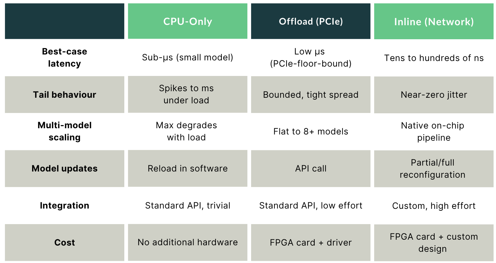
As the table above summarises, many production deployments use a mix: CPU-only for risk models and position management where occasional microsecond tails are acceptable, FPGA offload for medium-complexity alpha models where consistent low latency matters more than absolute minimum latency, and inline for the most latency-critical signal generation where sub-microsecond determinism is a hard requirement.
The Full Stack
This series has traced one argument across three layers:
Model structure determines the range of possible execution paths and their memory access patterns. Bounding tree depth and balancing memory footprints across processing units converts an unpredictable latency distribution into a bounded one.
Numerical representation determines how much memory the model occupies and whether compressed inference is numerically safe. Quantising thresholds at training time eliminates the pathological errors that post-training compression produces. Analytically computing leaf bit-widths prevents overflow without sacrificing the footprint reduction that makes quantisation worthwhile.
Compute architecture determines whether the remaining variance can be eliminated entirely, and at what cost. Optimised CPU inference is fast at the median but exposes tail risk under concurrent load. Offload accelerators remove tail spikes but add PCIe latency. Inline accelerators remove data movement from the hot path and replace it with deterministic digital logic that executes identically on every input.
Each layer has a ceiling set by the layers below it. Optimising the model on a general-purpose processor leaves software-level variance in place. Offloading to an accelerator removes that variance but leaves PCIe latency. The inline architecture removes the last movable floor.